

Want to hide the unused areas in Excel and focus only on the cells that contain your data? Follow the simple steps in this guide to keep your worksheet clean and distraction-free.
If you’ve ever opened a Microsoft Excel workbook and noticed that the columns, rows, or scrollbars are missing, there’s usually a simple explanation: the workbook’s author has hidden part of the worksheet. This can help users focus on the main working area without unnecessary distractions. When an Excel worksheet appears to be missing key elements, the author may have changed certain worksheet settings or view options to keep attention on the data.
In this tutorial, I’ll show you how to hide or disable several Excel worksheet elements and options so you can keep the focus on your working area. The process is straightforward and takes only a few moments to set up. I’m using Microsoft 365 Desktop on a 64-bit Windows 10 system, but the same steps generally work with older desktop versions of Excel. In Excel for the web, you can also turn off gridlines and row and column headings.
Why hide unused areas in Excel?
You might normally hide a row or column to keep sensitive data, formulas, or other information out of view. But why hide the rest of the worksheet? One reason is to limit what users can see or modify. By hiding everything except the main working area, you can create a cleaner interface while keeping supporting data and formulas out of sight.
Another useful reason is to make an Excel worksheet behave more like a dashboard. Dashboards are increasingly popular because they let viewers interact with reports, filter information, and explore charts without directly changing the underlying data.
If you want your Excel worksheet to work more like an interactive dashboard, hiding unused rows, columns, scrollbars, and other traditional worksheet elements can create a cleaner and more focused experience.
Whether your goal is to protect data or reduce visual distractions, hiding unused space and other worksheet elements can make Excel easier to work with. However, hiding rows and columns has one important side effect: it can shift the working area from its original position. For example, if you hide all the unused rows and columns, your main working area will move to the top-left corner of the worksheet instead of remaining centered.
That may not be an issue depending on how you use the spreadsheet. If you want to keep the working area centered, however, there’s another approach: turn off the gridlines. It’s worth noting that several of the techniques covered in this guide, including disabling gridlines, don’t technically hide worksheet elements. Instead, they turn off the display of certain worksheet properties and options to create a cleaner workspace.
Hiding columns and rows in Excel
Hiding unused rows and columns is an effective way to keep users focused on the information that matters. It can also prevent unnecessary navigation around empty areas of a worksheet. For dashboards, this technique can create a cleaner, more polished appearance that feels complete and professional.
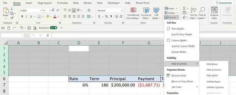
For this example, we’ll use the sample worksheet shown in Figure A. It contains a small working area surrounded by a large amount of unused space, which can encourage users to click or navigate beyond the intended area.
Figure A
How to hide unused rows in Excel
To hide the unused rows in your worksheet, follow these steps:
- Click a cell in the first unused row above your working area, then press Shift + Spacebar to select the entire row. In the example worksheet, select a cell in row 1.
- Press Ctrl + Shift + Down Arrow to select all rows from the selected row through the bottom of the worksheet.
- If the selection includes the header row, such as row 6, hold Shift and press the Up Arrow to remove that row from the selection.
- Select the Home tab on the Excel ribbon.
- In the Cells group, click Format, select Hide & Unhide, and then choose Hide Rows (Figure A). Alternatively, right-click the selected rows and choose Hide. You can also use the keyboard shortcut Ctrl + 9 to hide the selected rows.
Hiding the unused rows above the work area moves the work area to the top of the sheet, as shown in Figure B. This is the displacement issue I mentioned earlier.
Figure B

Repeat the steps above to select all the rows below the work area. Begin by clicking a cell in row 8. Figure C shows the results.
Figure C

Hide the unused columns
Next, you can hide the columns that aren’t part of your working area:
- Click any cell in column A.
- Press Ctrl + Down Arrow to move to the bottom of the column, or simply click the column header to select the entire column.
- Press Ctrl + Shift + Right Arrow to extend the selection across columns B and C.
- If Excel includes the first column of your working area in the selection, hold Shift and press the Right Arrow to remove it from the selection.
- In the Cells group, click Format, select Hide & Unhide, and then choose Hide Columns. You can also right-click the selected columns and choose Hide, or press Ctrl + 0.
Repeat these steps starting with a cell in column I to hide the unused columns on the other side of the working area.
As shown in Figure D, the working area now appears in the top-left corner of the worksheet. Although the unused rows and columns are hidden from view, you can still unhide them later if you need to make changes.

How to unhide rows and columns in Excel
To unhide all rows and columns in a worksheet, click the Select All button at the intersection of the row and column headers. This selects the entire worksheet. You can then use Ctrl + Shift + 9 to unhide rows and Ctrl + Shift + 0 to unhide columns.
How to hide worksheet elements in Excel
If moving the working area to the top-left corner, as shown in the previous example, doesn’t suit your needs, you can create a similar effect by turning off other worksheet elements, such as gridlines. This approach keeps the working area in place while making the surrounding empty space less noticeable.
To hide gridlines in Excel, follow these steps:
- Click the View tab.
- In the Show group, clear the Gridlines checkbox (Figure E).
Figure E
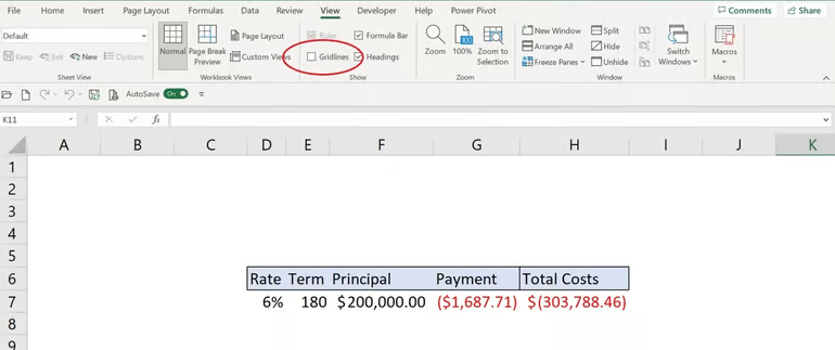
The gridlines are gone. This simple visual change will help the viewer move straight to the work area and stay there. Admittedly, it’s still white space, but the absence of the gridlines is a good start. However, the view still displays a few other sheet elements that you might want to inhibit. Next, let’s look at hiding header rows and the formula bar.
Hide header rows and the formula bar in Excel
Even with the gridlines turned off, the worksheet can still look unmistakably like an Excel spreadsheet. Hiding the row and column headings along with the formula bar can create a cleaner, more focused interface and encourage users to stay within the intended working area.
For this step, you’ll disable the headings and formula bar using the same View tab you used to hide the gridlines. Click the View tab, then clear the Formula Bar and Headings checkboxes in the Show group. The result is shown in Figure F.
Figure F
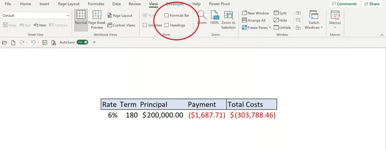
At this stage, users who are less familiar with Excel are less likely to navigate beyond the intended working area.
Even when the row and column headings are hidden, you can still select those cells and make changes to the worksheet. You can add or remove rows and columns as needed. In Figure F, for example, I inserted one column and two rows to position the working area more centrally.
Keep in mind that the Formula Bar is an application-level setting. This means that when you or your users open another Excel workbook, the Formula Bar will remain hidden. Because of this, you may want to leave it enabled, particularly if other users may not know how to turn it back on.
Hide the sheet tabs in Excel
Sheet tabs make it easy to switch between different worksheets within the same Excel workbook. If you want to create a more focused interface, you can also hide these tabs.
To turn off the display of sheet tabs, follow these steps:
- Click the File tab.
- Select Options from the left-hand pane.
- In the Excel Options window, click Advanced.
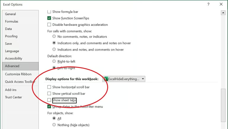
- Under Display Options for This Workbook, clear the first three checkboxes, as shown in Figure G. You can also disable the horizontal and vertical scroll bars while you’re here if you want to create an even cleaner workspace.
Figure G
- Click OK.
You can also hide or show the ribbon when needed, but Excel will most likely open the workbook with the ribbon visible. Like the Formula Bar, the ribbon is controlled by an application-level setting, so its display may carry over to other workbooks you open.
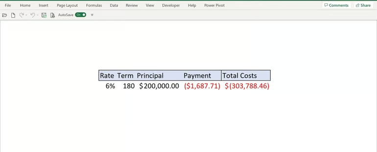
That’s it. Your worksheet is now set up with fewer visual distractions and a more focused working area. Figure H shows the final result: a simple, streamlined sheet that keeps attention on the content that matters.
Figure H
Restoring your original display
You’ve changed several Excel display settings, but each one is easy to restore. The entire process should take only a few minutes. To return the worksheet to its original appearance, simply repeat the steps described above in reverse order.
Moving toward Excel’s protection features
If you need to hide the Formula Bar and Ribbon automatically, you can use the Workbook_Open() event procedure. This procedure runs when the workbook is opened, allowing you to apply those display settings automatically. You can then restore them with the BeforeClose() event procedure when the workbook is closed.
The techniques covered in this tutorial are essentially a visual workaround. In many situations, they may be all you need, and they can give a worksheet a clean, professional appearance. However, hiding worksheet elements does not protect the cells or prevent users from accessing or changing the underlying data.
If your goal is to actually restrict access or prevent unwanted changes, use Excel’s built-in worksheet and workbook protection features instead.
Here are 8 SEO-friendly FAQs for the article:
Frequently Asked Questions
How do I hide unused rows and columns in Excel?
Select the unused rows or columns, right-click the selection, and choose Hide. You can also use Excel’s Home > Format > Hide & Unhide options.
How do I hide gridlines in an Excel worksheet?
Go to the View tab and clear the Gridlines checkbox in the Show group. This removes the visible grid pattern from the worksheet.
Can I hide the row and column headings in Excel?
Yes. Open the View tab and uncheck Headings in the Show group to hide the row numbers and column letters.
How can I hide the Formula Bar in Excel?
Go to View > Show and clear the Formula Bar checkbox. Keep in mind that this is an application-level setting and can affect other workbooks you open.
How do I hide sheet tabs in Excel?
Go to File > Options > Advanced, then find Display Options for This Workbook and clear the option that displays sheet tabs.
Does hiding rows and columns protect my Excel data?
No. Hiding worksheet elements only changes what users see. It does not prevent someone from accessing or modifying the hidden data. Use Excel’s Protect Sheet or Protect Workbook features when actual protection is required.
How do I restore hidden rows and columns in Excel?
Select the surrounding rows or columns, right-click the selection, and choose Unhide. You can also use Excel’s Hide & Unhide commands to restore them.
Can I make an Excel worksheet look like a dashboard?
Yes. Hiding unused rows and columns, turning off gridlines and headings, and removing unnecessary interface elements can create a cleaner, dashboard-like appearance while keeping the focus on the working area.
Conclusion
Hiding unused rows, columns, gridlines, headings, and other worksheet elements can give your Excel spreadsheet a cleaner, more focused appearance. These techniques are especially useful when you want users to concentrate on a specific working area or make a worksheet feel more like a dashboard.
Keep in mind that these settings are primarily for presentation and convenience, not data security. If you need to prevent users from viewing or changing important information, use Excel’s built-in protection features. With the right combination of display settings and protection tools, you can create a professional worksheet that is both easy to use and appropriately secured.
